Fantasy Shop 🐉⚔️ RAG Assistant 🛠️ crafted with Gemma and Rust 🦀

Today’s goal is to build an assistant for heroes who need to choose appropriate weapons for their adventures.

Before you will continue reading please watch short introduction:

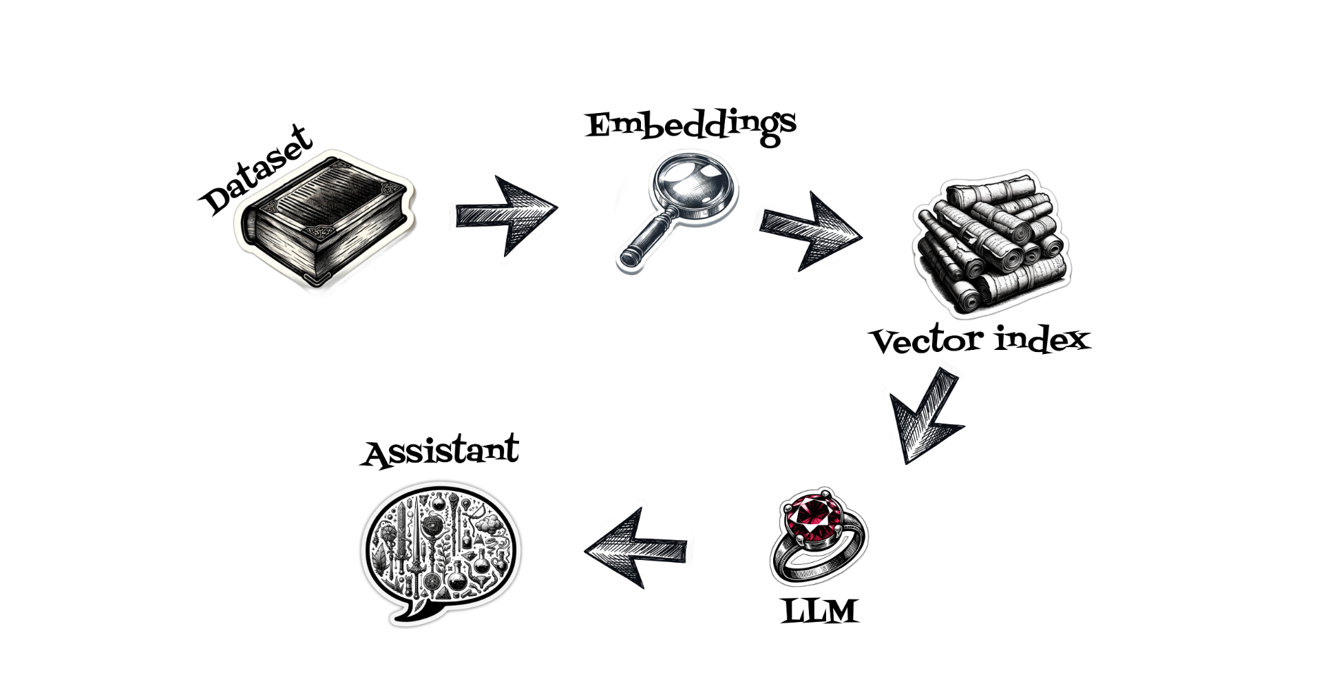
To develop our RAG-s solution, we will go through several steps: collecting and preparing a dataset, calculating embeddings, choosing an appropriate vector database, and finally, using an open-source large language model to build an assistant.

In the first step, we will collect a dataset, our dataset will be in Delta Lake format. To read it, we will use two Python packages that are built with Rust under the hood: Polars, which is a blazing-fast dataframe package, and delta-rs, which simplifies reading Delta tables without Spark.

FantasyAssistantPrep.ipynb

import polars as pl

table_path="../data/fantasy-library"
df=pl.read_delta(table_path)
df = df.with_columns(('For '+pl.col('Scenario')+' you should use '+pl.col('Advice')).alias('Combined'))
print(df)

To read a Delta table, we can simply use the read_delta method. Our delta contains two columns: Scenario and Advice. We will create an additional context column called Combined, which is simply a concatenation of the Scenario and Advice columns.

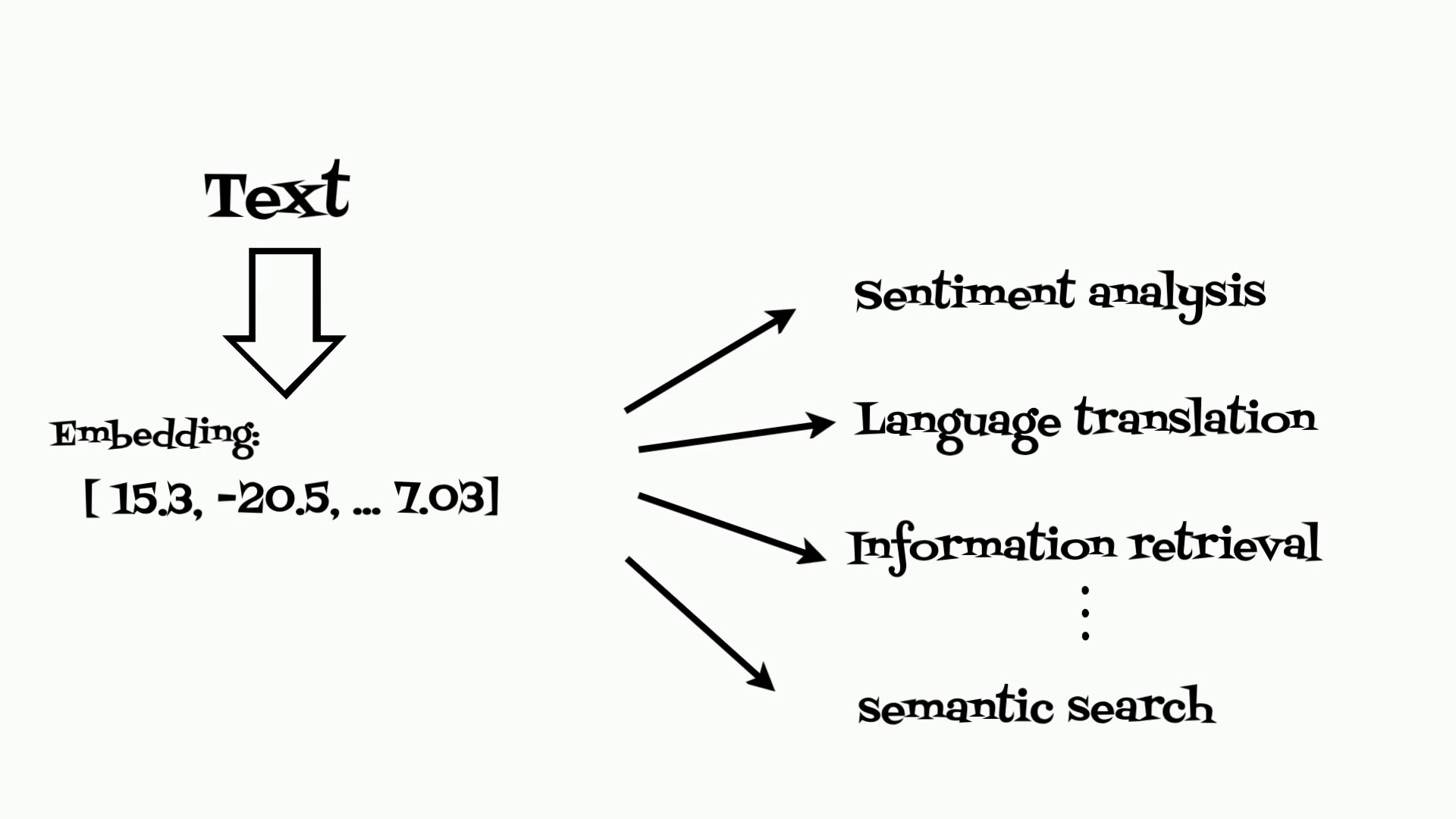
Now it’s time to calculate embeddings, which are multidimensional vectors calculated, for example, from text. To do this, we will use the E5 small model together with the Candle library.

Now it’s time to write some code in Rust. We will use the candle_transformers library to create an E5Model struct and add two methods. The first will download the model from Hugging Face, and the second will calculate embeddings for provided texts.

adventures/src/lib.rs

pub struct E5Model {
    pub model: BertModel,
    pub tokenizer: Tokenizer,
    pub normalize_embeddings: Option<bool>,
}

impl E5Model {
    pub fn load() -> Result<E5Model> {
        ...
    }

    pub fn forward(&self, input: Vec<String>) -> Result<Vec<Vec<f32>>> {
        ...
    }

We would like to use our Rust code in Python; thus, we will use the additional PyO3 maturing packages. In our case, we will wrap our Rust code with the Python Adventures module and Adventures class. After compilation, we are ready to import our adventures module and calculate embeddings for our contexts.

adventures-py/src/lib.rs

#[pymodule]
#[pyo3(name = "adventures")]
fn adventures(_py: Python, m: &PyModule) -> PyResult<()> {
    #[pyclass]
    pub struct Adventures {
        model: E5Model,
    }

    #[pymethods]
    impl Adventures {
        #[new]
        pub fn new() -> Self {
            let model = E5Model::load().unwrap();
            Self { model }
        }

        pub fn embeddings(&self, input: Vec<String>) -> PyResult<Vec<Vec<f32>>> {
            let embeddings = self.model.forward(input).unwrap();
            Ok(embeddings)
        }
    }

    impl Default for Adventures {
        fn default() -> Self {
            Self::new()
        }
    }

    m.add_class::<Adventures>()?;
    Ok(())
}

notebooks/FantasyAssistantPrep.ipynb

import adventures

a = adventures.Adventures()

items = []
for combined_text in df['Combined']:
    emb = a.embeddings([combined_text])
    items.append({"item": combined_text, "vector": emb[0]})

items

Now it’s time to choose a vector database where we will store our embeddings. To do this, we will use the LanceDb database. We can simply use the Python API to create a fantasy vectors table and create an index for it.

import lancedb
import numpy as np
uri = "/tmp/fantasy-lancedb"
db = lancedb.connect(uri)

tbl = db.create_table("fantasy_vectors", data=items)
tbl.create_index(num_partitions=256, num_sub_vectors=96)

Now we can confirm that we are able to use the created index to search for the most appropriate context. For example, in the first step, we calculate embeddings for “Adventure with a dragon” text. Then we search for the most appropriate context.

import lancedb

emb = a.embeddings(["Adventure with a dragon"])
db = lancedb.connect("/tmp/fantasy-lancedb")
tbl = db.open_table("fantasy_vectors")
df = tbl.search(emb[0]) \
    .limit(1) \
    .to_list()


df[0]["_distance"]

It is time for the large language model. In our case, we will use the Google Gemma model. Currently, Gemma models are published in two sizes: two billion and seven billion parameters. Additionally, we can use the instruct model type, which offers a specific turns prompt format that can be very helpful when building an assistant and wanting to keep the conversation context.

<start_of_turn>user
What is a good place for adventure ?<end_of_turn>
<start_of_turn>model
desert canyon.<end_of_turn>
<start_of_turn>user
What can I do in desert canyon ?<end_of_turn>
<start_of_turn>model

In our case, we will use the model with two billion parameters. Again, we will use the Rust Candle project to create a GemmaModel struct and a load method implementation. We aim to improve the user experience and, instead of creating a simple request-response method, we will use an additional async stream Rust library to stream text generated by the model.

adventures/src/lib.rs

pub struct GemmaModel {
    pub model: Model,
    pub device: Device,
    pub tokenizer: Tokenizer,
    pub logits_processor: LogitsProcessor,
    pub repeat_penalty: f32,
    pub repeat_last_n: usize,
}

impl GemmaModel {
    #[allow(clippy::too_many_arguments)]
    pub fn load(
        base_repo_id: &str,
        model_endpoint: Option<String>,
        seed: u64,
        temp: Option<f64>,
        top_p: Option<f64>,
        repeat_penalty: f32,
        repeat_last_n: usize,
        hf_token: Option<String>,
    ) -> Result<GemmaModel> {
        ...
    }
}

We have already collected the data, calculated embeddings, and indexed them into the LanceDb database. Now it’s time to create a microservice that will expose a chat POST method where our heroes’ team will send prompts. Inside the microservice, we will calculate embeddings using the E5 model, then search for the most appropriate context, build a large language model prompt in instruct format, and finally stream generated responses from the Gemma model to the heroes.

To build the microservice, we will use the Actix web framework.

During application start, we will load the Gemma model, E5 model, and additionally, we will create a LanceDb table object. For the Gemma model, we need to provide our Hugging Face token, which confirms that we have accepted the Gemma model license.

adventures/src/main.rs

static GEMMA_MODEL: OnceCell<Arc<Mutex<GemmaModel>>> = OnceCell::new();
 
//...
 
let model = GemmaModel::load(
    base_repo_id: GEMMA_2B_REPO_ID,
    model_endpoint: None,
    seed: 299792458,
    temp: Some(0.8),
    top_p: None,
    repeat_penalty: 1.1,
    repeat_last_n: 64,
    hf_token,
)
.unwrap();
 
GEMMA_MODEL.set(Arc::new(Mutex::new(model))).is_ok();

static E5_MODEL: OnceCell<Arc<Mutex<E5Model>>> = OnceCell::new();
 
//...
 
let e5_model = E5Model::load().unwrap();
 
E5_MODEL.set(Arc::new(Mutex::new(e5_model))).is_ok();

	static LANCEDB_TABLE: OnceCell<Arc<Mutex<lancedb::Table>>> = OnceCell::new();
 
//...
 
let uri = "/tmp/fantasy-lancedb";
let db = connect(uri).execute().await.unwrap();
let tbl = db.open_table("fantasy_vectors").execute().await.unwrap();
 
LANCEDB_TABLE.set(Arc::new(Mutex::new(tbl))).is_ok();

Inside the chat post method for request prompts, we will find the context which will cover calculating embeddings using the E5 model and searching for the most appropriate context.

adventures/src/main.rs

	pub async fn chat(
    request: web::Json<PromptRequest>,
    gemma_state: web::Data<GemmaState>,
) -> Result<impl Responder, Box<dyn Error>> {
    let context = find_context(request.prompt.to_string()).await.unwrap();
    let prompt = build_prompt(request.prompt.to_string(), context)
        .await
        .unwrap();
 
    let mut model = GEMMA_MODEL.get().unwrap().lock().await;
    model.model.clear_kv_cache();
 
    let mut tokens = model
        .tokenizer
        .encode(prompt.clone(), true)
        .map_err(anyhow::Error::msg)?
        .get_ids()
        .to_vec();
 
    let stream_tasks = stream! {
	
        for index in 0..request.sample_len {
            // ...

            yield Ok::<Bytes, Box<dyn Error>>(byte);
        }
	
    };
 
    Ok(HttpResponse::Ok()
        .content_type("text/event-stream")
        .streaming(Box::pin(stream_tasks)))
}

Now we are ready to build an instruct prompt using a simple template. Finally, we will pass the instruct prompt to the Gemma model and stream results. In this case, we run the Gemma model on CPU..

Additionally to improve solution prerformance we will use a model quantization process, which reduces model weights precision.

In the next step, we will use another open-source large language model, Mistral, with seven billion parameters which use 4-bit quantization. We will use the Candle library to load the model in gguf format, but in this case, we will use CUDA to run it on a GPU card.

adventures/src/lib.rs

pub struct QuantizedModel {
    pub model: ModelWeights,
    pub tokenizer: Tokenizer,
    pub device: Device,
}

impl QuantizedModel {
    pub fn load() -> Result<QuantizedModel> {
        //let base_repo_id = ("TheBloke/CodeLlama-7B-GGUF", "codellama-7b.Q4_0.gguf");
        let base_repo_id = (
            "TheBloke/Mistral-7B-Instruct-v0.2-GGUF",
            "mistral-7b-instruct-v0.2.Q4_K_S.gguf",
        );
        let tokenizer_repo = "mistralai/Mistral-7B-Instruct-v0.2";

        //...

        let device = Device::new_cuda(0).unwrap();

        //...
    }
}

Text transmutation - recipe for semantic search with embeddings

In the rapidly evolving area of data science and natural language processing (NLP), the ability to intelligently understand and process textual information is crucial. In this article I will show how to create a semantic search aplication using the Candle ML framework written in Rust, coupled with the E5 model for embedding generation.

Before you will continue reading please watch short introduction:

Text embeddings are at the heart of modern natural language processing (NLP). They are the result of transforming textual data into a numerical form that machines can understand.

To calculate embeddings I will use the E5 model (arxiv2212.03533) from Hugging Face to generate text embeddings.

E5 name comes from embeddings from bidirectional encoder representations. Model was trained on Colossal Clean text Pairs from heterogeneous semi-structured data sources like: Reddit (post, comment), Stackexchange (question, upvoted answer), English Wikipedia (entity name + section title, passage), Scientific papers (title, abstract), Common Crawl (title, passage), and others.

To run the E5 model I will use the Candle ML framework written in Rust. Candle supports a wide range of ML models including: Whisper, LLama2, Mistral, Stable Diffusion and others. Moreover we can simply compile and use Candle library inside WebAssembly to calculate text embeddings.

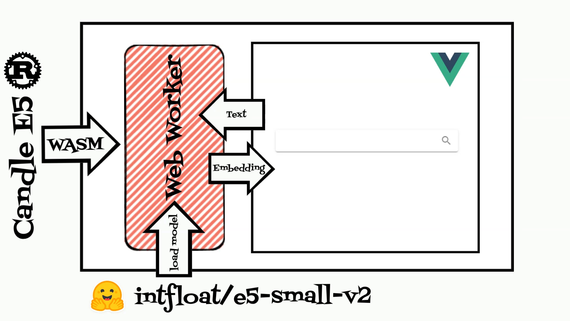
To demonstrate the power of these embeddings, I have created a simple search application. The application contains two parts: rust code which is compiled to WebAssembly and Vue web application.

The rust code is based on the candle Web Assembly example and expose model struct which loads the E5 model and calculates embeddings. Compiled rust struct is used in the Vue typescript webworker.

The web application reads example recipes and calculates embeddings for each.

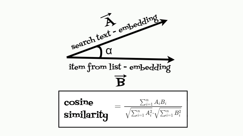
When user inputs a text application calculates embedding and search the recipe from the list that matches the best, the cosine similarity is used for this purpose.

Cosine similarity measures the cosine of the angle between two vectors, offering a way to judge how similar two texts are in their semantic content.

For handling larger datasets, it becomes impractical to compute cosine similarity for each phrase individually due to scalability issues. In such cases, utilizing a vector database is a more efficient approach.

Application code is available here: https://github.com/onceuponai-dev/stories-text-transmutation The rust part is based on Candle example

You can also quickly test model on: https://stories.onceuponai.dev/stories-text-transmutation/

Tiny LLama: Compact LLM with WebAssembly

Tiny LLama is an ambitious initiative aimed at pretraining a language model on a dataset of 3 trillion tokens. What sets this project apart is not just the size of the data but the efficiency and speed of its processing. Utilizing 16 A100-40G GPUs, the training of Tiny LLama started in September and is planned to span just 90 days.

Before you will continue reading please watch short introduction:

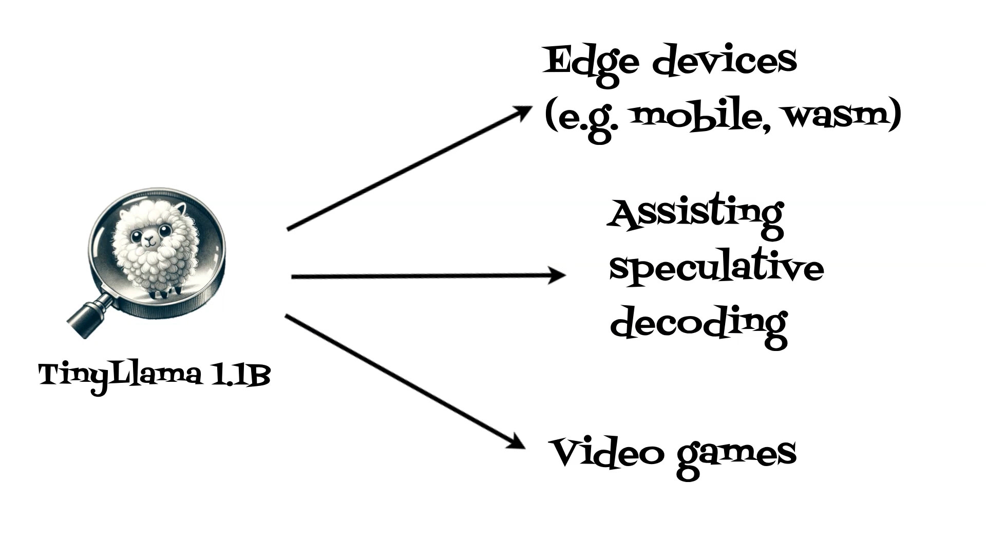
The compactness of Tiny LLama is its standout feature. With only 1.1 billion parameters, it is uniquely tailored for scenarios where computational and memory resources are limited. This makes it an ideal solution for edge devices.

For ease, I’ve prepared a Docker image containing all the necessary tools, including CUDA, mlc-llm, and Emscripten, which are crucial for preparing the model for WebAssembly.

Dockerfile:

 FROM alpine/git:2.36.2 as download

RUN git clone https://github.com/mlc-ai/mlc-llm.git --recursive /mlc-llm

FROM nvidia/cuda:12.2.2-cudnn8-devel-ubuntu22.04

RUN apt update && \
    apt install -yq curl git cmake ack tmux \
        python3-dev vim python3-venv python3-pip \
        protobuf-compiler build-essential


RUN python3 -m venv /opt/venv
ENV PATH="/opt/venv/bin:$PATH"
RUN python3 -m pip install --pre -U -f https://mlc.ai/wheels mlc-chat-nightly-cu122 mlc-ai-nightly-cu122

RUN apt install gcc
COPY --from=download /mlc-llm /opt/mlc-llm

RUN cd /opt/mlc-llm && pip3 install .

RUN apt-get install git-lfs -yq

ENV TVM_HOME="/opt/venv/lib/python3.10/site-packages/tvm/"

RUN git clone https://github.com/emscripten-core/emsdk.git /opt/emsdk
RUN cd /opt/emsdk && ./emsdk install latest

ENV PATH="/opt/emsdk:/opt/emsdk/upstream/emscripten:/opt/emsdk/node/16.20.0_64bit/bin:/opt/venv/bin:$PATH"
RUN cd /opt/emsdk/ && ./emsdk activate latest
ENV TVM_HOME=/opt/mlc-llm/3rdparty/tvm

RUN cd /opt/mlc-llm/3rdparty/tvm \
  && git checkout 5828f1e9e \
  && git submodule init \
  && git submodule update --recursive \
  && make webclean \
  && make web


RUN python3 -m pip install auto_gptq>=0.2.0 transformers

CMD /bin/bash

To build docker image we need to run:

docker build -t onceuponai/mlc-llm .

Now we are ready to run container:

docker run --rm -it --name mlc-llm -v $(pwd)/data:/data --gpus all onceuponai/mlc-llm

and execute mlc-llm command:

python3 -m mlc_llm.build --hf-path TinyLlama/TinyLlama-1.1B-Chat-v0.6  --target webgpu --quantization q4f32_0 --use-safetensors

where (Documentation): hf-path - is huggingface model name in this case TinyLlama/TinyLlama-1.1B-Chat-v0.6 target - is platfrom for which we prepare the model available options:

• auto (will detect from cuda, metal, vulkan and opencl)
• metal (for M1/M2)
• metal_x86_64 (for Intel CPU)
• iphone
• vulkan
• cuda
• webgpu
• android
• opencl

quantization - is quantization mode: available options: quantization: qAfB(_0) A - number of bits for weights B - number of bits for activations available options: autogptq_llama_q4f16_0, autogptq_llama_q4f16_1, q0f16, q0f32, q3f16_0, q3f16_1, q4f16_0, q4f16_1, q4f16_2, q4f16_ft, q4f32_0, q4f32_1 q8f16_ft, q8f16_1

In our case we will use webgpu target and q4f32_0 quantization to obtaind wasm file and converted model. I have shared several converted models on HuggingFace and Github.

Model can be simply used on web application.

Example typescript code is available here: https://github.com/onceuponai-dev/stories-thumbellama

You can also quickly test model on: https://stories.onceuponai.dev/stories-thumbellama/

Transform Your Coding Journey: Interactive Cheat Sheets with LLM Assistance

Cheat sheets are common companions in the journey through programming. They are incredibly helpful, offering quick references.

But what if we could take them a step further? Imagine these cheat sheets not just as static helpers, but as dynamic, interactive guides with the power of large language models. These enhanced cheat sheets don’t just provide information; they interact, they understand, and they assist. Let’s explore how we can make this leap.

Before you will continue reading please watch short introduction:

In the first step I have built Vue web application with responsive cheatsheet layout.

Next, I have brought Python into the browser using the Pyodide library. Pyodide is a port of CPython to WebAssembly. This means that we can run Python code right in the web browser, seamlessly integrating live coding examples and real-time feedback into cheatsheets.

The final, and perhaps the most exciting step, was adding LLM genie, our digital assistant. Using the mlc-llm library, I have embedded a powerful large language models into the web application. Currently we can choose and test several models like: RedPajama, LLama2 or Mistral. First and foremost, the LLM model, is designed to run directly in your browser on your device. This means that once the LLM is downloaded, all its processing and interactions happen locally, thus its performance depends on your device capabilities. If you want you to test it on my website:

https://www.onceuponai.dev/

Here, you can test the interactive cheat sheets and challenge the LLM with your code.

Data anonymization with AI

Data anonymization is the process of protecting private or sensitive information by erasing or encrypting identifiers that link an individual to stored data. This method is often used in situations where privacy is necessary, such as when sharing data or making it publicly available. The goal of data anonymization is to make it impossible (or at least very difficult) to identify individuals from the data, while still allowing the data to be useful for analysis and research purposes.

Before you will continue reading please watch short introduction:

I have decided to create a library which will help to simply anonymize data with high-performance. That’s why I have used Rust to code it. The library will use three algorithms which will anonymize data. Named Entity Recognition method enables the library to identify and anonymize sensitive named entities in your data, like names, organizations, locations, and other personal identifiers.

Here you can use existing models from HuggingFace for different languages for example:

• dslim bert-base-NER for english
• clarin FastPDN for polish

The models are based on external libraries like pytorch. To avoid external dependencies I have used rust tract library which is a rust onnx implementation.

To use models we need to convert them to onnx format using the transformers library.

import os
import transformers
from transformers import AutoModelForMaskedLM, AutoTokenizer, AutoModelForTokenClassification
from transformers.onnx import FeaturesManager
from pathlib import Path
from transformers import pipeline

model_id='dslim/bert-base-NER'
tokenizer = AutoTokenizer.from_pretrained(model_id)
model = AutoModelForTokenClassification.from_pretrained(model_id)

feature='token-classification'

model_kind, model_onnx_config = FeaturesManager.check_supported_model_or_raise(model, feature=feature)
onnx_config = model_onnx_config(model.config)

output_dir = "./dslim"
os.makedirs(output_dir, exist_ok=True)

# export
onnx_inputs, onnx_outputs = transformers.onnx.export(
        preprocessor=tokenizer,
        model=model,
        config=onnx_config,
        opset=13,
        output=Path(output_dir+"/model.onnx")
)

print(onnx_inputs)
print(onnx_outputs)
tokenizer.save_pretrained(output_dir)

Now we are ready to use the NER algorithm. We can simply run docker images with a yaml configuration file where we define an anonymization pipeline.

pipeline:
  - kind: ner
    model_path: ./dslim/model.onnx
    tokenizer_path: ./dslim/tokenizer.json
    token_type_ids_included: true
    id2label:
      "0": ["O", false]
      "1": ["B-MISC", true]
      "2": ["I-MISC", true]
      "3": ["B-PER", true]
      "4": ["I-PER", true]
      "5": ["B-ORG", true]
      "6": ["I-ORG", true]
      "7": ["B-LOC", true]
      "8": ["I-LOC", true]

docker run -it -v $(pwd):/app/ -p 8080:8080 qooba/anonymize-rs server --host 0.0.0.0 --port 8080 --config config.yaml

For the NER algorithm we can configure if the predicted entity will be replaced or not. For the example request we will receive an anonymized response and replace items.

curl -X GET "http://localhost:8080/api/anonymize?text=I like to eat apples and bananas and plums" -H "accept: application/json" -H "Content-Type: application/json"

Response:

{
    "text": "I like to eat FRUIT_FLASH0 and FRUIT_FLASH1 and FRUIT_REGEX0",
    "items": {
        "FRUIT_FLASH0": "apples",
        "FRUIT_FLASH1": "banans",
        "FRUIT_REGEX0": "plums"
    }
}

If needed we can deanonymize the data using a separate endpoint.

curl -X POST "http://localhost:8080/api/deanonymize" -H "accept: application/json" -H "Content-Type: application/json" -d '{
    "text": "I like to eat FRUIT_FLASH0 and FRUIT_FLASH1 and FRUIT_REGEX0",
    "items": {
        "FRUIT_FLASH0": "apples",
        "FRUIT_FLASH1": "banans",
        "FRUIT_REGEX0": "plums"
    }
}'

Response:

{
    "text": "I like to eat apples and bananas and plums"
}

If we prefer we can use the library from python code in this case we simply install the library. And we can use it in python.

We have discussed the first anonymization algorithm but what if it is not enough ? There are two additional methods. First is Flush Text algorithm which is a fast method for searching and replacing words in large datasets, used to anonymize predefined sensitive information. For flush text we can define configuration where we can read keywords in separate file where each line is a keyword or in the keyword configuration section.

The last method is simple Regex where we can define patterns which will be replaced.

We can combine several methods and build an anonymization pipeline:

pipeline:
  - kind: ner
    model_path: ./dslim/model.onnx
    tokenizer_path: ./dslim/tokenizer.json
    token_type_ids_included: true
    id2label:
      "0": ["O", false]
      "1": ["B-MISC", true]
      "2": ["I-MISC", true]
      "3": ["B-PER", true]
      "4": ["I-PER", true]
      "5": ["B-ORG", true]
      "6": ["I-ORG", true]
      "7": ["B-LOC", true]
      "8": ["I-LOC", true]
  - kind: flashText
    name: FRUIT_FLASH
    file: ./tests/config/fruits.txt
    keywords:
    - apple
    - banana
    - plum
  - kind: regex
    name: FRUIT_REGEX
    file: ./tests/config/fruits_regex.txt
    patterns:
    - \bapple\w*\b
    - \bbanana\w*\b
    - \bplum\w*\b

Remember that it uses automated detection mechanisms, and there is no guarantee that it will find all sensitive information. You should always ensure that your data protection measures are comprehensive and multi-layered.